
Parametric regression model for survival data: Weibull regression model as an example
Author’s introduction: Zhongheng Zhang, MMed. Department of Critical Care Medicine, Jinhua Municipal Central Hospital, Jinhua Hospital of Zhejiang University. Dr. Zhongheng Zhang is a fellow physician of the Jinhua Municipal Central Hospital. He graduated from School of Medicine, Zhejiang University in 2009, receiving Master Degree. He has published more than 35 academic papers (science citation indexed) that have been cited for over 200 times. He has been appointed as reviewer for 10 journals, including Journal of Cardiovascular Medicine, Hemodialysis International, Journal of Translational Medicine, Critical Care, International Journal of Clinical Practice, Journal of Critical Care. His major research interests include hemodynamic monitoring in sepsis and septic shock, delirium, and outcome study for critically ill patients. He is experienced in data management and statistical analysis by using R and STATA, big data exploration, systematic review and meta-analysis.

Abstract: Weibull regression model is one of the most popular forms of parametric regression model that it provides estimate of baseline hazard function, as well as coefficients for covariates. Because of technical difficulties, Weibull regression model is seldom used in medical literature as compared to the semi-parametric proportional hazard model. To make clinical investigators familiar with Weibull regression model, this article introduces some basic knowledge on Weibull regression model and then illustrates how to fit the model with R software. The SurvRegCensCov package is useful in converting estimated coefficients to clinical relevant statistics such as hazard ratio (HR) and event time ratio (ETR). Model adequacy can be assessed by inspecting Kaplan-Meier curves stratified by categorical variable. The eha package provides an alternative method to model Weibull regression model. The check.dist() function helps to assess goodness-of-fit of the model. Variable selection is based on the importance of a covariate, which can be tested using anova() function. Alternatively, backward elimination starting from a full model is an efficient way for model development. Visualization of Weibull regression model after model development is interesting that it provides another way to report your findings.
Keywords: Survival analysis; parametric model; Weibull regression model
Submitted May 20, 2016. Accepted for publication Jun 23, 2016.
doi: 10.21037/atm.2016.08.45
Introduction
While semi-parametric model focuses on the influence of covariates on hazard, fully parametric model can also calculate the distribution form of survival time. Advantages of parametric model in survival analysis include: (I) the distribution of survival time can be estimated; (II) full maximum likelihood can be used to estimate parameters; (III) residuals can represent the difference between observed and estimated values of time; (IV) estimated parameters provide clinically meaningful estimates of effect (1). There are a variety of models to be specified for accelerated failure time model including exponential, Weibull and log-logistic regression models. In this article, Weibull regression model is employed as an example to illustrate parametric model development and visualization.
Weibull regression model
Before exploring R for Weibull model fit, we first need to review the basic structure of the Weibull regression model. The distribution of time to event, T, as a function of single covariate is written as (1):

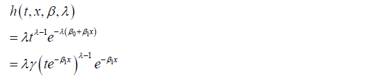
where β1 is the coefficient for corresponding covariate, ε follows extreme minimum value distribution G(0, σ)and σ is the shape parameter. This is also called the accelerated failure-time model because the effect of the covariate is multiplicative on time scale and it is said to “accelerate” survival time. In contrast, the effect of covariate is multiplicative on hazard scale in the proportional hazard model. The hazard function of Weibull regression model in proportional hazards form is:
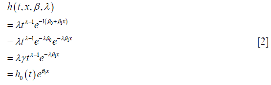
where 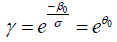 ,
, 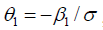 , and the baseline hazard function is
 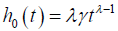 . σ is a variance-like parameter on log-time scale.
  is usually called a scale parameter. Parameter λ is a shape parameter. Parameter θ1 has a hazard ratio (HR) interpretation for subject-matter audience.
The accelerated failure-time form of the hazard function can be written as:
Weibull regression model can be written in both accelerated and proportional forms, allowing for simultaneous description of treatment effect in terms of HR and relative change in survival time [event time ratio (ETR)] (2).
Fitting Weibull regression model with R
The survreg() function contained in survival package is able to fit parametric regression model. Let’s first load the package into the workspace. To build a Weibull regression model, the dist argument should be set to a string value “weibull”, indicating the distribution of response variable follows Weibull distribution. The summary() function is to print content of the returned object of class survreg.

The output first recalls the structure of the Weibull regression model, including the covariates. Next, the coefficients of each covariate are shown, together with standard error and P values. Scale is an important parameter in Weibull regression model and is shown in the following line. A log likelihood test shows that the model is significantly better than null model (P=1.4e–06). However, the estimated coefficients are not clinically meaningful. That is why Weibull regression model is not widely used in medical literature. Since Weibull regression model allows for simultaneous description of treatment effect in terms of HR and relative change in survival time, ConvertWeibull() function is used to convert output from survreg() to more clinically relevant parameterization. The function is contained in SurvRegCensCov package and we need to install it first.

The first table of the output displays parameters of the Weibull regression model. Lambda and gamma are scale and shape parameters of Weibull distribution. The estimate for each covariate is different from that displayed in the value column of the summary() output. The relationship can be described by an equation β = −α/σ, where α is parameter for each of the covariate and σ is the scale (2). In our example, β is the estimate in the first table of the ConvertWeibull() output and α is displayed in the output of summary(wei.lung). The second table shows the HR and corresponding 95% confidence interval. The last table displays the ETR and its 95% confidence interval. Female reduces the risk of death compared to male by 42% (HR =0.58), and female significantly increases the survival time by approximately 50% (ETR =1.49). Although HR is more widely reported in medical literature and is familiar to clinicians, ETR may be easier to understand.
Alternatively, the Weibull regression model can be fit with WeibullReg() function. In essence, it is the combination of survreg() and ConvertWeibull().

Adequacy of Weibull model
Weibull model with categorical variables can be checked for its adequacy by stratified Kaplan-Meier curves. A plot of log survival time versus log[–log(KM)] will show linear and parallel lines if the model is adequate (3).

Figure 1 is the Weibull regression diagnostic plot showing that the lines for male and female are generally parallel and linear in its scale.

Weibull regression model with eha package
An alternative way to model Weibull regression model is via eha package. This package provides a variety of functions for Weibull regression model. Let’s now first install the package and load it into the workspace.

The argument of weibreg() function is similar to that of the survreg(). The coefficient of covariates in the above output is the HR in log scale. Thus, the exponentiation of coefficient gives the HR.
Hazard, cumulative hazard, density and survivor functions can be plotted from the output of a Weibull regression model.

Figure 2 is the graphical display of the output of Weibull regression model. The fn argument specifies the functions to be plotted. It receives a vector of string values, choosing from “haz”, “cum”, “den” and “sur”. The newdata argument specifies covariate values at which to plot the function. If covariates are left unspecified, the default value is the mean of the covariate in the training dataset. In the example, four plots were drawn at age of 80, 60, 40 and 20 years old (in the order from left to right and from top to bottom). The sex and ph.ecog variables were set at values of 2 and 3, respectively.

Graphical goodness-of-fit test
The eha package has a function check.dist() to test the goodness-of-fit by graphical visualization. It compares the cumulative hazards functions for non-parametric and parametric model, requiring objects of “coxreg” and “phreg” as the first and second argument.

The solid line is the parametric Weibull cumulative hazard function and the dashed line is non-parametric function. It appears that the parametric function fits well to the semi-parametric function (Figure 3). Note that non-parametric model is closer to the observed data because no function is assumed for the baseline hazard function.

Variable selection and model development
Like generalized linear model development (4), it is essential to include statistically important and clinically relevant covariates into the model in fitting parametric regression model. While clinical relevance is judged by clinical expertise, the statistical importance is determined by software. The anova() function tests the statistical importance of a covariate, interaction and non-linear terms. The function reports Chi-square statistics and associated P value. Also, it provides dot charts depicting the importance of variables in the model.

In the example, we included all available covariates into the model to rank their statistical importance. This is often the case in real research setting that researchers have no prior knowledge on which variable should be included. The first argument of psm() function is a formula describing the response variable and covariates, as well as interaction between predictors. The output of anova() includes variable names, Chi-square statistics, degree of freedom and p-value. Dot chart is drawn with generic function plot(). It appears that meal.cal is the least important variable and ph.ecog is the most important one (Figure 4). Some pre-specified rules can be applied to inclusion/exclusion of variables (4).

Alternatively, model development can be done with backward elimination on covariates. This method starts with a full model that included all available covariates and then applies Wald test to examine the relative importance of each one. Statistical significance level for a covariate to stay in a model can be specified. R provides a function fastbw() to perform fast backward variable selection.

The first argument of fastbw() receives an object fit by psm(). The rule argument defines stopping rule for backward elimination. The default is Akaike’s information criterion (AIC). If P value is used as the stopping rule (rule=“p”), the significance level for staying in a model can be modified using sls argument (sls =0.1 for example). The output shows that variables meal.cal, sex, pat.karno and wt.loss are eliminated from the model based on AIC. Sometimes if you want to retain a covariate in the model based on clinical judgment, the force argument can be employed. It passes a vector of integers specifying covariates to be retained in the model. Intercept is not counted.
Visualization of Weibull regression model
Weibull model can be used to predict outcomes of new subjects, allowing predictors to vary. In Weibull regression model, the outcome is median survival time for a given combination of covariates. We first use Predict() to calculate median survival time in log scale, then use ggplot() function to draw plots.

In the example, an interaction term sex*age is specified. We let variable age to vary between 20 to 80 years old. Both male and female, and all four levels of ph.ecog are considered. Figure 5 shows the output of ggplot() function. The effect of age on survival time is dependent on sex. While older age is associated with shorter survival time in the male, it is associated with longer survival time in the female.
Figure 5 visualizes relationship between covariates. Occasionally, investigators may be interested in survivor and/or hazard functions of individuals with given covariate patterns. The smoothSurv package provides functions for this purpose. Similarly to the previous model building strategy, we first fit a model including interaction terms between sex and age.


A matrix object of cov is created representing 4 patients whose survival time is unknown and the treating physician wants to make a prediction based on Weibull regression model. The number of columns of the matrix should be equal to the number of covariates in the model, including interaction terms.

The output is a series of plots showing survivor, cumulative distribution, hazard and density functions (Figure 6). Cov1 to cov4 are indicators of four patients with given covariate patterns. Important parameters of the model are displayed at the bottom of each plot.

Acknowledgements
None.
Footnote
Conflicts of Interest: The author has no conflicts of interest to declare.
References
- Hosmer DW Jr, Lemeshow S, May S. editors. Applied Survival Analysis, 2nd ed. New York: John Wiley & Sons, Inc., 2008:1.
- Carroll KJ. On the use and utility of the Weibull model in the analysis of survival data. Control Clin Trials 2003;24:682-701. [Crossref] [PubMed]
- Klein JP, Moeschberger ML. editors. Survival Analysis: Techniques for Censored and Truncated Data, 2nd ed. New York: Springer, 2005:1.
- Zhang Z. Model building strategy for logistic regression: purposeful selection. Ann Transl Med 2016;4:111. [Crossref] [PubMed]

